Colour by code in Excel with VBA - Part 1

Want a quick way to highlight cells by their content ?  Read on! 

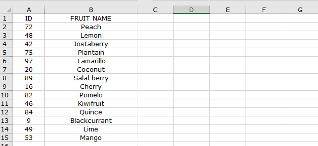
Before:

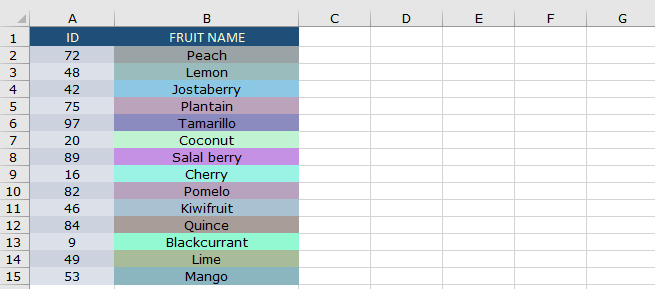
After:

 As of the writing of this article, Excel doesn't have much by way of separating out text fields by colour, despite having had a variety of numeric gradient formatting for a number of years.

RGB

All colours on screens are made of RGB pixels , from this you can mix any colour you like:

For example -  Cyan is a mixture of Green and Blue, Purple a mixture of Red and blue, Grey is an even mix of all colours.

You can read up on it here : https://en.wikipedia.org/wiki/RGB_color_model

 We can use these components and conditionally mix them to create our background colours.

ASCII 

The next thing we need to know, is that every letter in the alphabet has a corresponding number - this is called an ASCII code.  In the standard ASCII set there are 255 characters, which includes, numbers, letters, punctuation and special non-printing characters.

RGB colour in Excel is stored as a range of 0-255 for each 'pot'   - if we just take the first, middle and last character from a string, and turn it into a colour, we get the below :

It works, but the colours are very dull. Clearly converting straight from ASCII to RGB isn't going to work.

So what now? 

We just need to be smarter about how we're applying the numbers.

In the standard ASCII set , the 26 Uppercase, 26 Lowercase and 10 numbers only a quarter of the possible ASCII codes, and represent a limited range, therefore we're not getting sufficient variance from simply applying them directly to a colour mix.

Instead what we need to do, is sort them into sets ( Upper, Lower and Numeric ) , from there, we can determine set upper and lower boundaries for that set, and with that fixed, we can calculate a generic position within that ranger, and return a value between 0 and 1. 

 First, what are the bounds?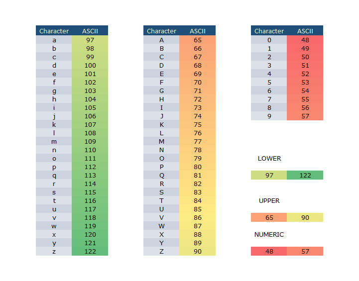   

So we have uppercase, running from 65 - 90 , lower from 97 -122 and numeric from  48-57 .

Our first function - lets take the character as an input, then return a float of range of 0-1 depending on which category it falls in  ( Upper, Lower or Numeric ) .

Here's the output  - side by side with the original- already the colours are looking more defined.

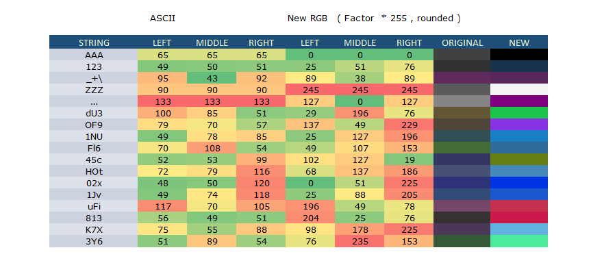Here's the code to return the factor float based on the cell text :

Function Alpha_Fact(INSTRE As String) As Double

Dim AscNum As Integer, RtnNum As Double

'UPPER CASE 65  90  26
'NUMERIC   48  57 10
'LOWER CASE   97  122 26

If Len(INSTRE) < 1 Then INSTRE = "AMZ"

AscNum = Asc(Left(INSTRE, 1))

Select Case AscNum
    
    ' ::: UPPER  :::::::
    Case 65 To 90
    RtnNum = (AscNum - 64) / 26
    
    ' ::: LOWER :::::::::::
    Case 97 To 122
    RtnNum = (AscNum - 96) / 26
    
    ' ::: NUMERIC :::::::::::::::
    Case 48 To 57
    RtnNum = (AscNum - 47) / 10
    
    ' ::: OTHER ::::::::::::::::::::::
    Case Else:
    RtnNum = Int((AscNum / 255) * 250) / 250

End Select

Alpha_Fact = RtnNum

In the below chart - just looking at the first half of the ASCII range, you can see how it works :

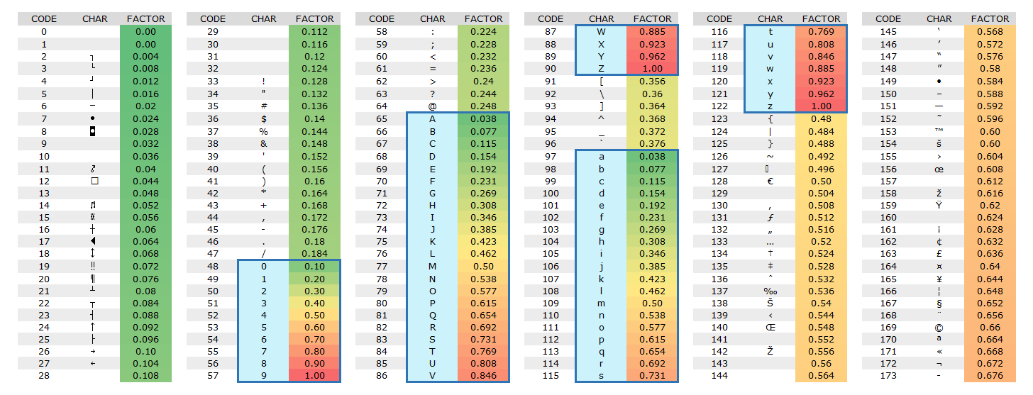Where it fits within a bracket ( upper / lower / numeric ) it returns  0-1 relative to that bracket, else it'll return 0-1 based on it's overall position in the range of 0-255. 

 Putting it all together 

Now we have our conditional range - its' now time to put it into a procedure to apply to ranges.

Sub ColourByText()



Dim Rr As Range, Cc As Range, DD As Range, cR, cG, cB As Double, CstrB As String
Dim Rnt, Gnt, Bnt As Double
Dim STL, STM, STR As String
Dim StrString As String
Dim MaxHue As Single, MaxRow As Long
Dim bSpecial As Boolean
Set Rr = Selection
bSpecial = False

For Each DD In Rr.Areas
    
    MaxRow = Last(1, DD)
    
    
    'MsgBox DD.Rows.count & "Max Row :" & MaxRow
    
    
    For Each Cc In DD
    
        bSpecial = False
        If Cc.Row > MaxRow Then Exit For
        
        StrString = Cc.text
        
        If StrString <> "" Then
        
        StrString = Trim(StringCleanNPC(StrString))
        
        STL = Left(StrString, 1)
            
            If Len(StrString) > 2 Then
                STM = Mid(StrString, Round(Len(Cc.text) / 2, 0), 1)
                Else: STM = STL
            End If
        
        STR = Right(StrString, 1)
        
        Rnt = Int(Alpha_Fact(Left(STM, 1)) * 96)
        Gnt = Int(Alpha_Fact(Left(STL, 1)) * 160)
        Bnt = Int(Alpha_Fact(Left(STR, 1)) * 96)
        
        '
        ':: special cases ::
        '
        
        Select Case UCase(StrString)
        
        Case "BREAK":
        Rnt = 254
        Gnt = 184
        Bnt = 156
        bSpecial = True
        
        Case "MATCH":
        Rnt = 157
        Gnt = 248
        Bnt = 132
        bSpecial = True
        
        Case "NO":
        Rnt = 254
        Gnt = 184
        Bnt = 156
        bSpecial = True
        
        Case "YES":
        Rnt = 157
        Gnt = 248
        Bnt = 132
        bSpecial = True
        
        Case "Y":
        Rnt = 254
        Gnt = 184
        Bnt = 156
        bSpecial = True
        
        Case "N":
        Rnt = 157
        Gnt = 248
        Bnt = 132
        bSpecial = True
        
        Case "---":
        Rnt = 180
        Gnt = 180
        Bnt = 220
        bSpecial = True
   
        End Select
        
        
        ':::  --Do nothing if empty - ::
        
        If Len(StrString) > 0 And bSpecial = False Then Cc.Interior.Color = RGB(140 + Rnt, 255 - Gnt, 140 + Bnt)
        If bSpecial Then Cc.Interior.Color = RGB(Rnt, Gnt, Bnt)
        
        
        End If
        
    Next Cc
Next DD

End Sub

 In the above, it'll analyse the first, middle and last letter of cell to return the factor 0-1 , with a slight bias towards green. 

There's also a conditional statement at the end, which, when specified, will assign a specific colour to a specific word, this is useful for generic columns with Y/N Yes/No True/False etc. ( Or names ) .

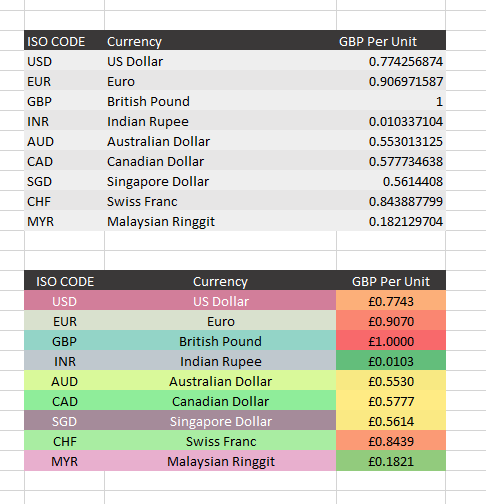
As an example of usage - here a quick currency char is spiced up by the automatic colours.  Where it's based on  content, and therefore deterministic - users will quickly be able to spot lines / items  by colour  ( for example, USD will always be Salmon coloured, GBP be Turquoise etc.   )