Vlookup vs Index-Match - a better way of searching.

So you want to vlookup some stuff, and it's going wrong huh?

You're frustrated by having to count along the column headings to find the right column number to return the data you need? 

Worry no more, there's a better way of finding things, and once you've mastered it, you'll never want to vlookup ( or hlookup ) again.

 To find out more about vlookup - check the microsoft page.  

 Here's an illustration of the primary reason vlookup is so limited :

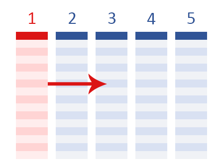
Can you spot it?   You can only go one way.. 

Now , here's an illustration of the Index-Match combination :

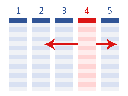
With an Index Match, you can go in any direction, you're no-longer bound by the limitations of having your search column ( and your result column ) having to be in a specific order before you can begin your lookups! 

What's wrong with Vlookup? Most of the time, nothing.

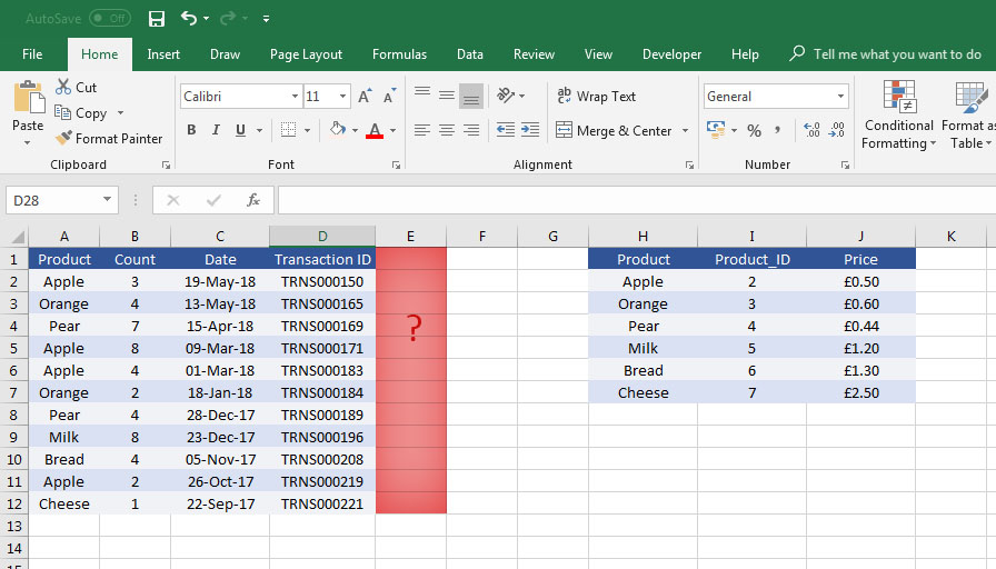
Here's an example of a typical need for a vlookup.  We have a list of transactions taking place, and another table of the prices of each of the items, but we need to find out the cost of the transaction. 

To find out the cost of the transaction, we need to look up the product, then return the price. 

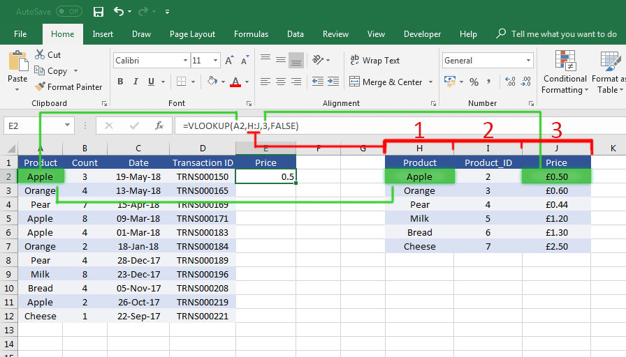
In the below example,  I'm searching for "Apple" Cell A2 in Column (1) of Range H:J, and returning the corresponding value from column 3 ( J ) .   It returns the value from J2, as this is the same row as "Apple" is found in Column 1 ( H ) . 

Vlookup always uses the first column of your range as the "lookup" range.

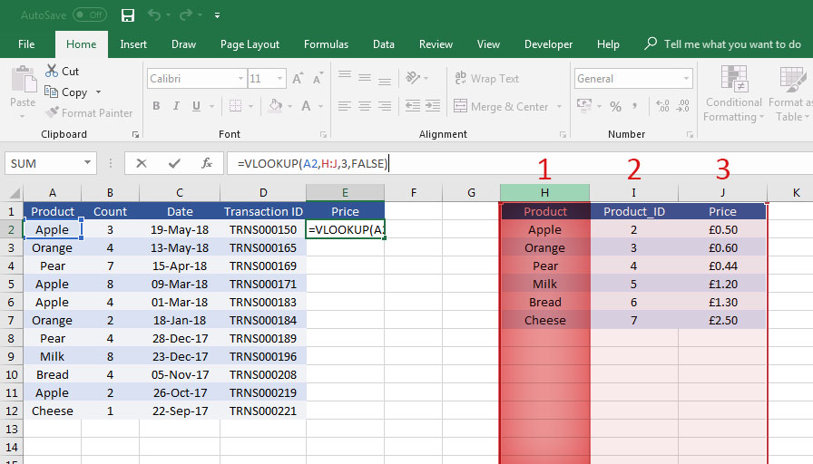
And here is how the results come back :

This is fine for most purposes, however, consider the following scenario :

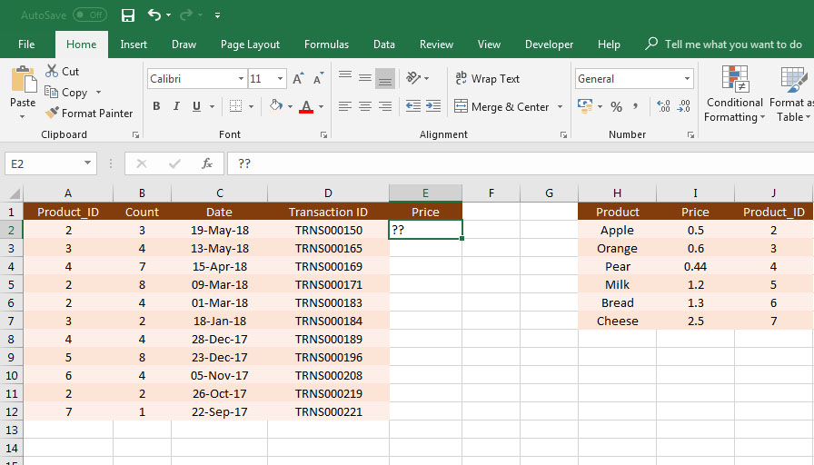Say you were not allowed to change the column order of the lookup table ( the sheet is on a workbook you can't edit), what then?

Introducing Index-Match!

It may look complicated at first, but it's very similar to vlookup, and best of all, you're not having to memorise column numbers to get your result. 

INDEX( Value Range  , MATCH( Search Value , Search Range , Search Type Flag ))

Where Index refers to the column you want to return the results from, and Match is the column you are searching for the specific search value.  The search flag we can get onto later, but for most purposes, this can be left as 0. 

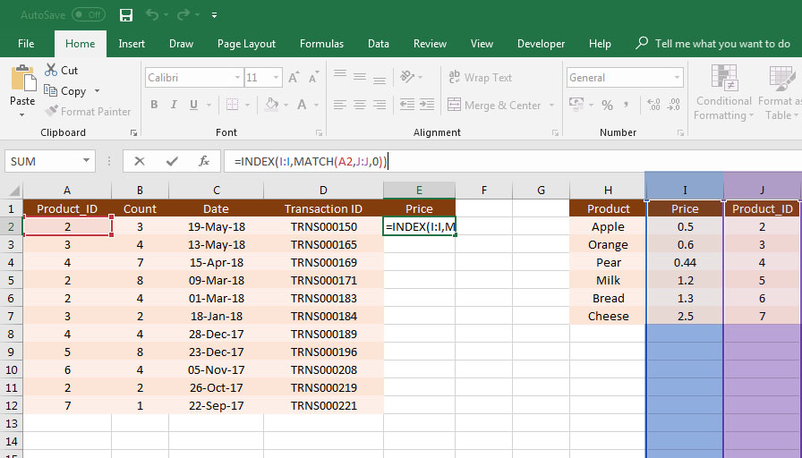But what about the cost of the apples? 

In this example, all we have to go off is a product ID , with no name or price, so lets put those both in.

First the product name, same as above, we search in column L for the Product_ID (Cell A2), and return the corresponding row from column J.  

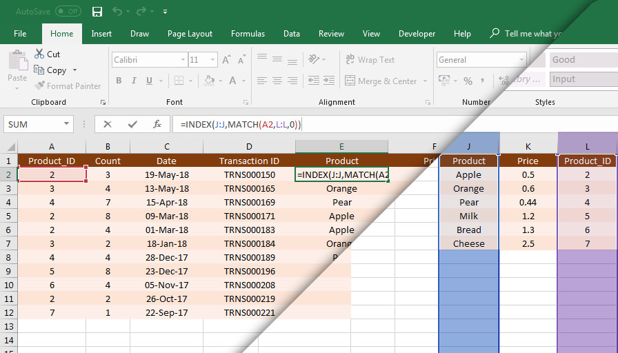
Then we do the same to lookup the price on column K

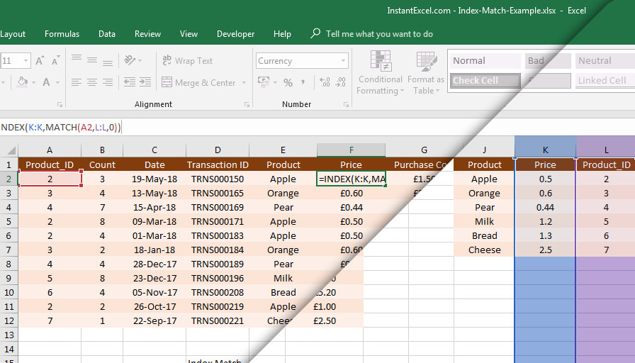
 So all we need to do now is multiply the count of items in the transaction by the price, like so :

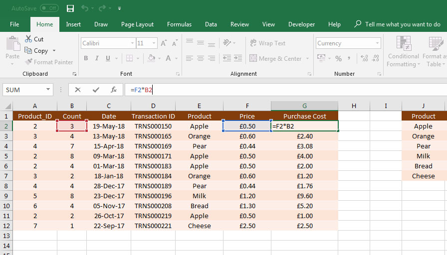
Is that it? 

For most people yes, but if you want to know more, read on!

Remember that 'flag' for match type, the one we just set to '0' ? 

For the most part you'll want to keep it at 0, but if you're working with numbers, you can use it to find approximate matches.  It's covered plenty elsewhere , so I won't go into detail, but for the purposes of text matching ( which is primarily what vlookups appear to be used for ) , just keep this as '0'

But I don't know if my Apple is Green or Red?

The boss wants to know the price of the apples in the order, but what if they're not Green?

This is where a wildcard ( * ) comes in. You're probably used them before, searching folders / google etc.
The only difference here, is with formulas in excel, you'll need to add double-quotes.

INDEX( Value Range  , MATCH( "*" & Search Value , Search Range , Search Type Flag ))

In the example below, we're searching column C for any text ending with Apple, the Wildcard ( * ), tells excel to ignore anything before the word apple, and match it.

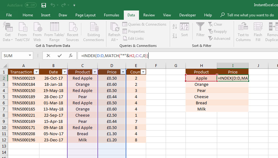So now we've found the price of the apples, red or not.

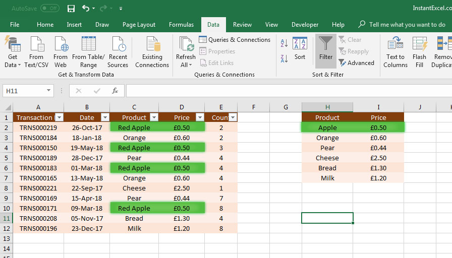
 ..and finally, the pitfalls of the wildcard. 

One thing to be aware of , as with anything involving partial matching, is you're sure when using a wildcard for whatever reason, that you're not potentially matching two different values.

In the below scenario, we have two different apples, and two different prices, the wildcard match simply pulls back the first matching result , but this isn't the true price of apples.
You can see Red apples are 50p, while the Green are 80p.

Saying all apples are 50p is now incorrect. 

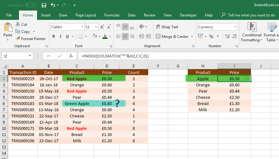This is where you'll need to explore other Excel functions, like MinIfs / AverageIfs / MaxIfs, if you want to find the most expensive apple, the average apple price etc.   

I'll be covering those functions in due course, but for now, I hope this has given you some insight into, and perhaps encouraged you to have a go with Index-Match. 

It's not as complicated as it looks, and is a lot more flexible than your favourite vlookups.

 TL:DR - Try for yourself - download the example workbook ( 21 kB ).